Plotting

This walkthrough covers the built-in plotting helpers in topo.plot and how to colour, compare and save figures. Every image below was produced by the code shown next to it, on the same example data as the step-by-step tutorial.

Plotting is built on matplotlib, which is installed by default.

Setup

We fit once and reuse the result for every plot:

import topo as tp
from data import load_cells

X, labels, label_names = load_cells(return_names=True)

tg = tp.TopOGraph(random_state=0)
tg.fit(X)

tg.fit computes the 2-D layouts; the plots below just draw them. Every topo.plot function returns a matplotlib Figure, so you can show it in a notebook or save it with fig.savefig(...).

1. A basic scatter

scatter draws a 2-D layout, one point per row, coloured by group:

fig = tp.plot.scatter(tg.TopoMAP, labels=labels, pt_size=6)

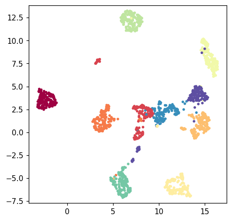
labels are mapped through a colormap (cmap, default "Spectral"). Pass any per-row array — integer groups here, or a continuous value (see §3).

2. Compare layouts side by side

tg.fit produces several layouts. Drawing them together makes it easy to pick the one that tells the clearest story. Here we use matplotlib directly on the embedding arrays:

import matplotlib.pyplot as plt

fig, axes = plt.subplots(1, 3, figsize=(15, 5))
for ax, (emb, title) in zip(
    axes,
    [(tg.TopoMAP, "TopoMAP"),
     (tg.msTopoMAP, "msTopoMAP"),
     (tg.TopoPaCMAP, "TopoPaCMAP")],
):
    ax.scatter(emb[:, 0], emb[:, 1], c=labels, s=5, cmap="Spectral")
    ax.set_title(title)
    ax.set_aspect("equal")
    ax.axis("off")

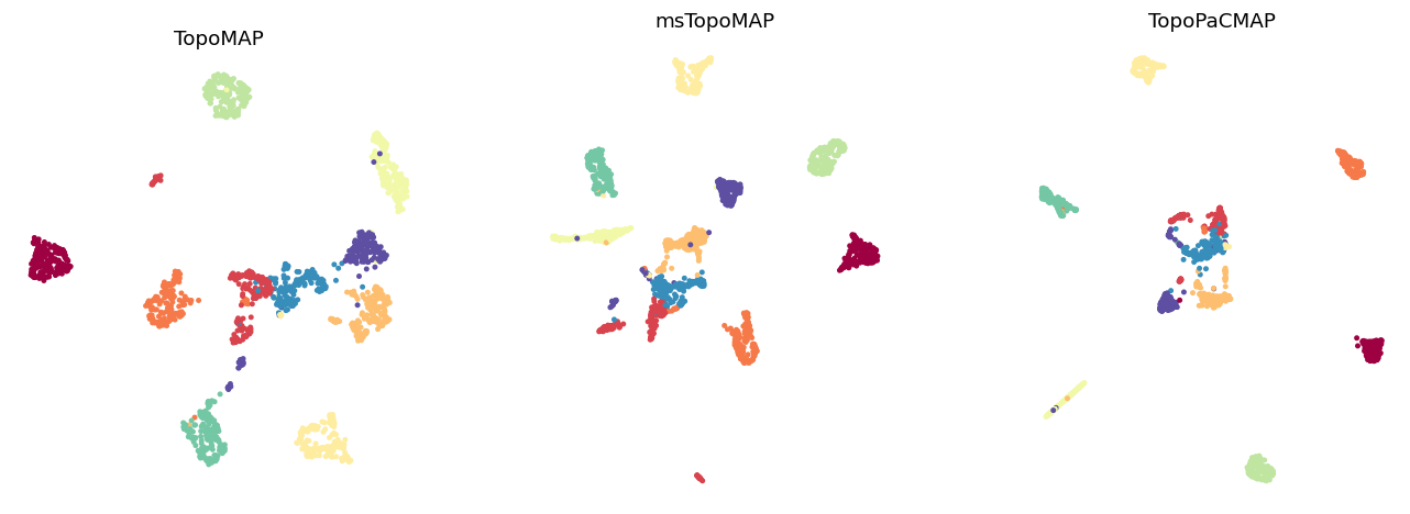
Each layout is just an (n_rows, 2) array, so anything you can do with matplotlib works directly.

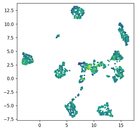
3. Colour by a continuous value

Instead of groups, colour by any per-row number — an expression level, a score, or here the total intensity of each row. Use a sequential colormap:

intensity = X.sum(axis=1)
fig = tp.plot.scatter(tg.TopoMAP, labels=intensity, pt_size=6, cmap="viridis")

4. The eigenspectrum (scree plot)

tg.eigenspectrum() shows how much structure each successive pattern carries — useful for judging how many components hold real signal:

fig = tg.eigenspectrum()

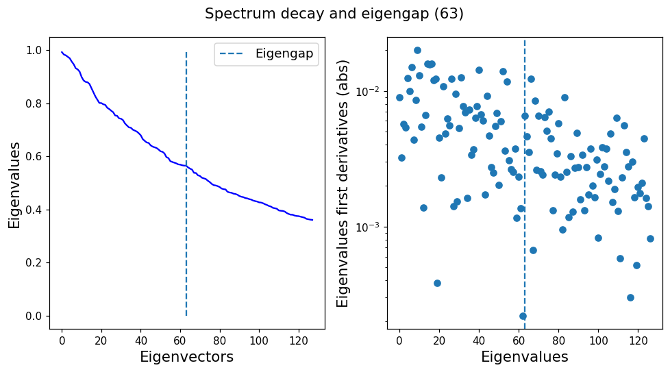
The dashed line marks the estimated eigengap, a rough cut between signal and the flat noise tail.

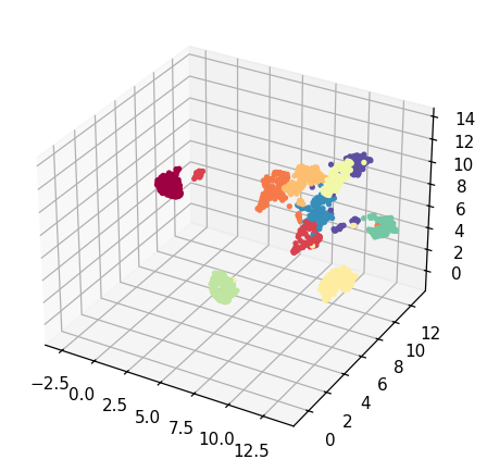
5. A 3-D scatter

Ask for a 3-component layout and draw it with scatter3d:

emb3d = tg.project(n_components=3, projection_method="MAP")
fig = tp.plot.scatter3d(emb3d, labels=labels, pt_size=6)

Saving figures

Every helper returns a Figure, so save in any format matplotlib supports:

fig = tp.plot.scatter(tg.TopoMAP, labels=labels)
fig.savefig("topomap.png", dpi=200, bbox_inches="tight")  # or .pdf, .svg

In a Jupyter notebook the figure also displays inline automatically.